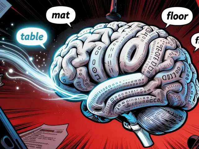
Imagine typing a question into an AI assistant and staring at a blank screen. One second passes. Then two. By the time you hit four seconds, your trust in the tool has already started to erode. In the world of interactive large language model applications, this delay isn't just annoying; it's fatal.
The difference between a chatbot that feels like a helpful colleague and one that feels like a broken appliance comes down to milliseconds. But here is the catch: Large Language Models (LLMs) are heavy, complex beasts. They don't just "think"; they process massive amounts of data sequentially. To make them feel instant, engineers have to work within strict latency budgets. These budgets define the maximum acceptable time from when a user hits "Enter" to when they see the first word appear on their screen.
If you are building or deploying an AI app today, understanding these constraints is non-negotiable. You can't just throw more GPUs at the problem without breaking the bank or creating new bottlenecks. Let's look at how to balance speed, cost, and quality so your application actually works for humans.
The Two Phases of LLM Inference
To manage latency, you first need to understand where the time goes. LLM inference isn't a single block of processing; it happens in two distinct phases with very different characteristics. Knowing this helps you target optimizations effectively.
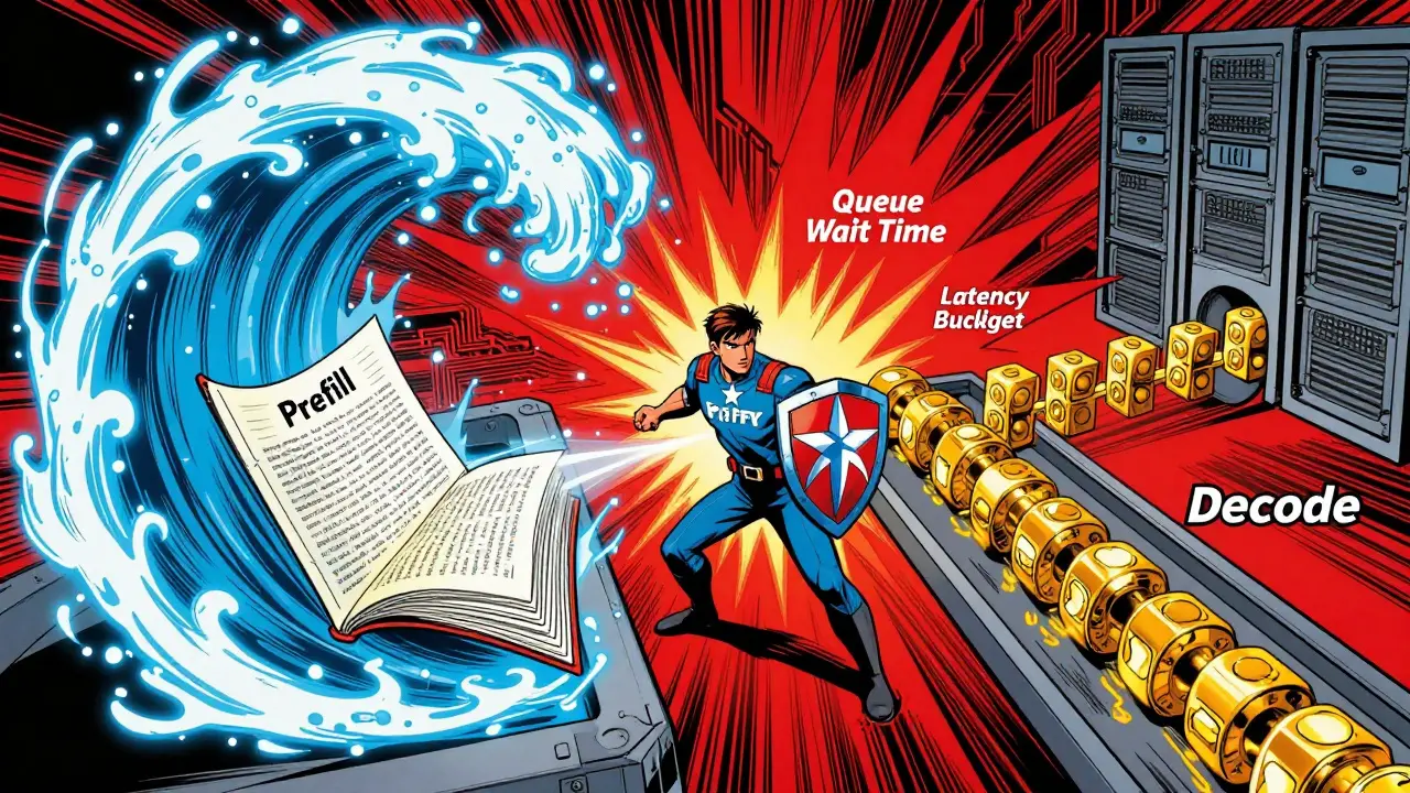
The Prefill Phase is what happens immediately after the user submits their prompt. The model reads the entire input-whether that's a short sentence or a 10,000-token document-and builds a Key-Value (KV) Cache. This phase is compute-bound, meaning it relies heavily on the GPU's raw calculation power. Because the model processes the whole prompt at once, this part is highly parallelizable. If your users send long prompts, this phase dominates the initial wait time.
The Decode Phase follows next. This is where the magic happens: generating tokens one by one. Unlike prefill, decode is sequential. The model cannot generate the second token until the first is done, and it must access the growing KV cache for every single step. This makes the decode phase memory-bandwidth bound. As the response gets longer, the KV cache grows, slowing down memory access. This creates an asymmetry: prefill is fast but expensive in compute, while decode is slow because it waits on memory.
For interactive apps, this split matters. If your app handles long-context queries (like summarizing legal documents), the prefill phase will dictate your initial latency. If it's a casual chat, the decode phase's speed determines how fluid the conversation feels.
Defining Your Latency Metrics
You can't improve what you don't measure. In LLM deployment, generic terms like "response time" are too vague. You need to track specific metrics that map directly to user perception.
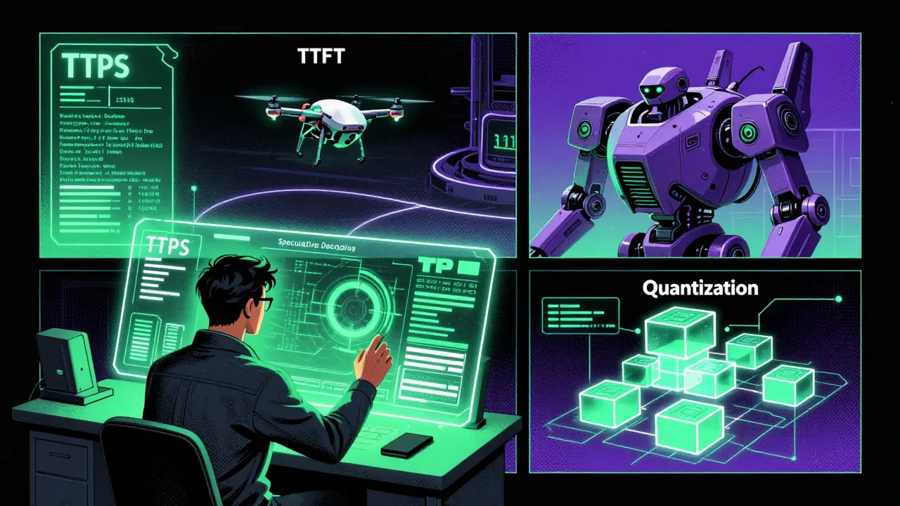
Time to First Token (TTFT) is the most critical metric for interactivity. It measures the time from request submission to the appearance of the very first character. Humans perceive responsiveness based on TTFT. If TTFT is under 500 milliseconds, the app feels instant. Between 500ms and 2 seconds, it feels normal. Beyond 2 seconds, users start to doubt if the system is working. TTFT is primarily driven by the prefill phase and the size of the model.
Tokens Per Second (TPS) measures the generation speed during the decode phase. While TTFT gets the user's attention, TPS keeps it. A high TPS means the text streams quickly, mimicking human typing speed. If TPS drops too low, the stream chugs, breaking immersion. TPS is constrained by memory bandwidth, not compute power.
There is also Inter-Token Latency (ITL), which is the time between individual tokens. High variance in ITL causes stuttering. For a smooth experience, you want consistent ITL, even if the average TPS is moderate.
| Metric | Phase | Primary Constraint | User Impact |
|---|---|---|---|
| TTFT | Prefill | Compute Power | Perceived Responsiveness |
| Tokens Per Second | Decode | Memory Bandwidth | Flow and Immersion |
| End-to-End Latency | Both | Total Processing Time | Task Completion Speed |
The Batching Dilemma: Throughput vs. Latency
One of the biggest traps in LLM deployment is batching. Batching multiple requests together improves GPU utilization and reduces cost per token. However, it introduces a direct trade-off: higher throughput often means higher latency for individual users.
When you batch requests, each request waits in a queue before being processed. Consider the Qwen 2.5 7B model. At a batch size of 1, latency might be around 976 milliseconds. Increase the batch size to 8, and the latency per request drops significantly due to better hardware efficiency, but the *wait time* for any single user increases because they are waiting for the batch to fill. Throughput gains show diminishing returns beyond certain batch sizes. Going from batch size 2 to 4 might double your throughput, but going from 16 to 32 yields smaller gains while potentially spiking tail latency.
For interactive applications, you cannot maximize batch size blindly. You need to tune parameters like `max_num_seqs` (maximum number of sequences in a batch) and `max_num_batched_tokens`. Higher concurrency raises Requests Per Second (RPS) by keeping GPUs busy, but excessive load increases TTFT and ITL. The goal is to find the "sweet spot" where GPU utilization is high enough to be cost-effective, but low enough to keep TTFT under your budget.
Architectural Optimizations for Speed
If tuning batching isn't enough, you need to change how the model computes. Several advanced techniques can stretch your latency budget without sacrificing quality.
Speculative Decoding is one of the most effective methods. Instead of the large model generating every token from scratch, a smaller, faster "speculator" model predicts several tokens ahead. The large model then verifies these predictions. If they are correct, the system skips the heavy computation for those tokens. This can reduce inference latency by 2x to 4x. It trades extra compute (for the speculator) for lower latency, which is a great deal if you have spare GPU capacity.
Quantization reduces the precision of model weights, allowing them to fit into less memory and process faster. For example, using MXFP4 quantization allows models like GPT OSS 20B to run on smaller GPU allocations (around 13.1 GB VRAM) compared to BF16 formats. While there is a slight risk to accuracy, modern quantization techniques maintain high quality while significantly boosting TPS by reducing memory bandwidth pressure.
Mixture of Experts (MoE) architectures offer another path. MoE models activate only a subset of parameters for each input. The GPT OSS 20B MoE model, for instance, has 20 billion total parameters but only activates 3.6 billion per forward pass. This sparse activation improves memory efficiency and allows for larger batch sizes before hitting memory limits. However, MoE introduces routing overhead, which can add complexity and sometimes negate latency benefits if not implemented carefully.
Model Selection and Cost Trade-offs
Your choice of model dictates your baseline latency. Smaller models are inherently faster. A 7B parameter model will almost always have a lower TTFT and higher TPS than a 70B model on the same hardware. For instance, smaller variants like GPT-4.1-mini are typically 5x faster than their larger counterparts. The trade-off is capability. Larger models follow instructions better and produce higher-quality reasoning.
Infrastructure costs compound this decision. Deploying a 109B parameter model might require three NVIDIA H100 GPUs with 80GB VRAM each. A 400B model could need ten such GPUs. These aren't just capital expenses; they translate to operational costs. A startup handling 10,000 requests per day with online RAG might spend $15,000 per month on a 109B model versus $30,000 for a 400B model. But remember, more GPUs don't always mean lower latency if the bottleneck is memory bandwidth during the decode phase.
Only smaller models (around 8B parameters) can reliably fit onto a single 80GB GPU. If your latency budget is tight and your use case allows for slightly lower reasoning depth, downsizing the model is the fastest way to gain performance.
Caching and Retrieval Strategies
In many interactive scenarios, especially Retrieval-Augmented Generation (RAG) apps, you are repeating work. If two users ask the same question about the same document, why run the inference twice? Caching frequently requested responses eliminates redundant computation, drastically cutting both cost and latency.
However, caching requires careful strategy. You need robust cache invalidation rules to ensure users get up-to-date information. For RAG systems, where prompts can be large (up to 10,000 tokens) but responses are short, caching the prefill results or the final answer can be transformative. Infrastructure tools like Bifrost help automate this by managing intelligent routing and caching layers, ensuring that identical or similar requests hit the cache rather than the GPU.
Practical Implementation Checklist
To build an interactive LLM app that respects latency budgets, follow these steps:
- Measure Baseline TTFT: Test your model with typical prompt lengths. Aim for under 1 second for best-in-class UX.
- Optimize Prompt Length: Trim unnecessary context. Every extra token in the prefill phase adds latency.
- Implement Speculative Decoding: Use a small draft model to accelerate generation if your hardware supports it.
- Tune Batch Sizes: Monitor tail latency, not just average throughput. Reduce batch size if P99 latency spikes.
- Use Quantization: Switch to FP8 or INT4 weights if accuracy tests pass, to relieve memory bandwidth pressure.
- Cache Aggressively: Implement semantic caching for RAG apps to avoid re-processing common queries.
What is a good Time to First Token (TTFT) for an interactive AI app?
Aim for under 500 milliseconds for an "instant" feel. Between 500ms and 2 seconds is generally acceptable for most users. Anything over 2 seconds risks losing user engagement as they begin to doubt the system's functionality.
Does increasing batch size always improve performance?
No. While batching increases throughput (requests per second), it often increases latency for individual users because they wait in a queue. There is a diminishing return point where adding more requests to a batch slows down memory access and increases tail latency.
How does speculative decoding reduce latency?
Speculative decoding uses a smaller, faster model to predict multiple tokens ahead. The larger, primary model then verifies these predictions. If correct, the system skips the heavy computation for those tokens, effectively trading extra compute for significant latency reductions (often 2x-4x).
Why is the decode phase slower than the prefill phase?
The prefill phase is parallelizable and compute-bound, allowing the GPU to process the entire prompt at once. The decode phase is sequential and memory-bandwidth bound. Each new token requires accessing the growing Key-Value (KV) cache, which becomes increasingly slow as the context length grows.
Can quantization affect the quality of LLM responses?
Yes, potentially. Quantization reduces the precision of model weights (e.g., from BF16 to FP8 or INT4). While modern techniques minimize loss, extreme quantization can lead to subtle errors in reasoning or instruction following. Always validate quality metrics after applying quantization.