
Have you ever asked an AI assistant a question about your company’s internal policies, only to get a confident but completely wrong answer? That moment of disappointment is what we call hallucination. It happens because Large Language Models (LLMs) are trained on static data from the past. They don’t know your latest product updates, your private customer records, or the new regulations that passed yesterday. Worse, they might just make things up to sound helpful.
This is where Retrieval-Augmented Generation, or RAG, comes in. Think of RAG as giving your AI a library it can actually read before answering. Instead of relying solely on its memory, the system first retrieves relevant facts from your own data sources-like databases, documents, or data lakes-and feeds them into the prompt. This grounds the AI in reality, drastically reducing hallucinations and ensuring your answers are accurate and up-to-date.
But how do you find the right fact among millions of documents in milliseconds? That’s the job of vector databases, embeddings, and smart indexing algorithms like HNSW. Let’s break down how this architecture works, why it matters for your business, and how to build it without getting lost in the technical weeds.
What Are Embeddings and Why Do They Matter?
To understand RAG, you first need to understand embeddings. An LLM doesn’t “read” text like you do. It sees numbers. An embedding is a mathematical representation of text, images, or other data converted into high-dimensional vectors-essentially long arrays of numbers. These numbers capture the semantic meaning of the content.
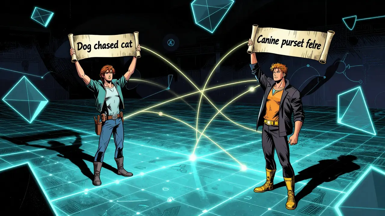
Imagine you have two sentences: "The dog chased the cat" and "A canine pursued a feline." To a human, these mean the same thing. To a basic keyword search engine, they share almost no words. But to an embedding model, these sentences will result in vectors that are very close together in mathematical space. This proximity signals similarity.
In a RAG system, the process starts by taking your domain-specific dataset and chunking it into smaller, semantic elements. You then use a specialized embedding model to compute a vector for each chunk. Popular choices include open-source models like all-MiniLM-L12-v2 from the SentenceTransformer package, which produces efficient 384-dimensional vectors, or cloud-native options like Amazon Titan Text Embedding v2 for production environments on AWS Bedrock.
When a user asks a question, their query is also turned into a vector using the exact same model. The system then searches for the vectors in your database that are closest to the query vector. This ensures consistency in the semantic space. If the embedding model changes between indexing and querying, the math breaks, and your retrieval accuracy plummets.
The Role of Vector Databases in RAG
You could store these vectors in a standard spreadsheet or a traditional relational database, but that would be painfully slow. Traditional databases are built for exact matching-finding a record where ID equals 123. They aren’t designed to calculate the distance between two points in a 384-dimensional space across millions of rows.
Vector databases are specifically architected for this workload. They serve as the long-term memory for your LLM, storing millions to billions of embeddings and retrieving the top-k nearest neighbors in milliseconds. Whether you use a purpose-built solution like Pinecone or an extension like Pgvector for PostgreSQL, the goal is the same: perform similarity searches efficiently.
Pgvector, for instance, adds a "vector" data type to PostgreSQL along with three query operators for similarity searching:
- Euclidean distance: Measures the straight-line distance between points.
- Cosine distance: Measures the angle between vectors, which is often better for text embeddings.
- Negative inner product: An alternative metric useful in specific contexts.
Most modern text embedding models are optimized for cosine similarity. It focuses on the orientation of the vectors rather than their magnitude, which aligns well with how semantic meaning is distributed in high-dimensional spaces.
HNSW Indexing: Speeding Up Search Without Sacrificing Accuracy
Here’s the problem with naive similarity search: if you have one million vectors, the database has to compare your query against all one million vectors to find the best match. This is called a brute-force search, and it takes seconds. In a real-time chat application, seconds feel like hours. Users bounce.
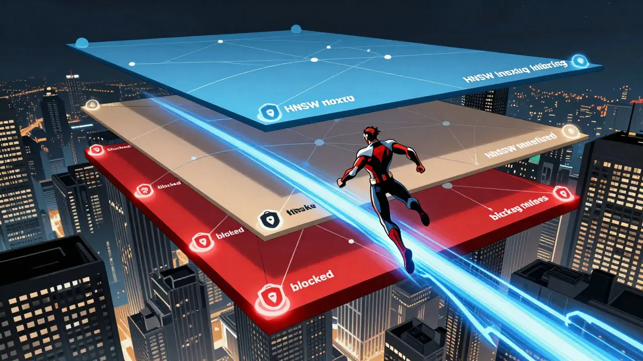
This is where Hierarchical Navigable Small World (HNSW) indexing saves the day. HNSW is a graph-based algorithm designed for approximate nearest neighbor (ANN) searches. Instead of checking every single vector, HNSW organizes your data into a multi-layered graph structure.
Think of it like navigating a city. The top layer of the graph has long-range connections that let you jump quickly across large distances to get near your destination. As you move down the layers, the connections become shorter and more detailed, allowing you to fine-tune your location until you land on the most similar vector.
The trade-off here is between speed and recall. Recall refers to how many of the truly relevant results you actually find. HNSW allows you to tune parameters to balance this. For most enterprise applications, the slight drop in theoretical perfection is worth the massive gain in speed.
Consider a real-world test case using Pgvector with one million rows of 384-dimensional embeddings. Building an HNSW index on this dataset took about 33 minutes. But once indexed, similarity search times dropped from several seconds per query to mere milliseconds. That’s a 100x+ performance improvement. This makes real-time RAG commercially viable.
Alternative Indexing Methods: IVFFlat vs. HNSW
HNSW isn’t the only game in town. Another common method is IVFFlat (Inverted File with stored vectors). IVFFlat uses geometric partitioning to break your vector space into small, queryable sub-indexes or clusters. When a query comes in, the system only searches the specific partitions that are likely to contain the answer, ignoring the rest.
So, which one should you choose? Here is a quick comparison:
| Feature | HNSW | IVFFlat |
|---|---|---|
| Search Speed | Very Fast (Milliseconds) | Fast (Depends on partitions) |
| Recall (Accuracy) | High (Tunable) | Moderate (Lower than HNSW) |
| Index Build Time | Slower | Faster |
| Memory Usage | Higher | Lower |
| Best For | Production apps requiring low latency | Larger datasets with less strict latency needs |
If you need the absolute fastest response times and can afford the extra memory and build time, HNSW is usually the winner. If you are dealing with massive datasets where even approximate clustering helps, IVFFlat might be a lighter option. Some advanced systems even combine methods using techniques like Reciprocal Rank Fusion (RRF) to boost relevance further.
Filtering: Adding Business Logic to Semantic Search
Semantic similarity is powerful, but it’s not enough on its own. Imagine a multi-tenant SaaS platform. Company A shouldn’t see the documents belonging to Company B, even if those documents are semantically similar to the query. Or consider compliance: you might want to exclude sensitive HR documents from general employee queries.
This is where filtering mechanisms come in. Vector databases allow you to constrain similarity searches based on metadata. Before or during the vector search, you apply filters like `tenant_id = '123'` or `document_type != 'confidential'`. This ensures that the retrieved results are not only semantically relevant but also contextually appropriate.
The challenge with filtering is performance. If you filter too aggressively, you might end up searching an empty subset of your index. Modern vector databases handle this by integrating metadata indexes alongside vector indexes, allowing for efficient filtered searches across large datasets without scanning the entire space.
Building Your RAG Pipeline: Step-by-Step
Implementing RAG requires careful architectural decisions. Here is a practical workflow based on industry best practices:
- Chunking: Break your source documents into manageable pieces. Too large, and you lose precision; too small, and you lose context. Aim for semantic completeness in each chunk.
- Embedding: Pass each chunk through your chosen embedding model (e.g., all-MiniLM-L12-v2). Store the resulting vectors along with the original text and metadata (like author, date, tenant ID).
- Indexing: Create an HNSW index on your vector column. Tune the `m` and `ef_construction` parameters if you’re using Pgvector to balance build speed and search quality.
- Query Processing: When a user asks a question, embed the query using the same model.
- Retrieval: Query the vector database for the top-k nearest neighbors, applying any necessary metadata filters.
- Generation: Append the retrieved chunks to your LLM prompt. Ask the LLM to answer the question based only on the provided context.
A pro tip: Keep your embeddings close to your source data. If you’re using PostgreSQL with Aurora ML, you can generate embeddings directly within the database using stored procedures. This eliminates the need to export data for transformation and keeps your pipeline simple and secure.
Common Pitfalls to Avoid
Even with the right tools, RAG implementations can fail if you ignore these common traps:
- Inconsistent Embedding Models: Never mix and match embedding models for indexing and querying. The vector spaces won’t align.
- Ignoring Chunk Size: Poor chunking leads to fragmented context. Experiment with different chunk sizes and overlap strategies.
- Overlooking Latency: Without proper indexing (like HNSW), your app will be too slow for users. Always benchmark your search times.
- Forgetting Filters: Security and privacy rely on metadata filters. Test them rigorously to prevent data leakage between tenants or roles.
RAG with vector databases is no longer just a research concept. It’s the backbone of reliable, enterprise-grade generative AI. By mastering embeddings, leveraging HNSW for speed, and applying strict filters, you can build AI applications that are not only smart but also trustworthy.
What is the main benefit of using HNSW over IVFFlat?
HNSW generally offers faster search speeds and higher recall (accuracy) compared to IVFFlat. While IVFFlat is faster to build and uses less memory, HNSW's graph-based structure allows for more precise navigation of the vector space, making it ideal for production applications requiring low-latency responses.
How does RAG reduce hallucinations in LLMs?
RAG reduces hallucinations by grounding the LLM's response in retrieved, factual data from your own knowledge base. Instead of generating answers from its pre-trained memory, which may be outdated or incorrect, the LLM uses the specific context provided in the prompt to formulate its response.
Why is cosine similarity preferred for text embeddings?
Cosine similarity measures the angle between two vectors, focusing on their orientation rather than their magnitude. For text embeddings, this is effective because it captures semantic relationships regardless of the length of the text chunks, making it robust for comparing documents of varying sizes.
Can I use PostgreSQL for vector storage?
Yes, by using extensions like Pgvector. Pgvector adds vector data types and indexing capabilities (including HNSW and IVFFlat) to PostgreSQL, allowing you to store and search embeddings directly within your existing relational database infrastructure.
What role do metadata filters play in RAG?
Metadata filters ensure that retrieved information meets specific business rules, such as user permissions, document confidentiality levels, or tenant isolation. They prevent the AI from accessing irrelevant or unauthorized data, enhancing both security and relevance.



Saranya M.L.
July 10, 2026 AT 23:17It is truly disheartening to see Western tech blogs attempting to explain the fundamentals of vector space mathematics as if it were a novel discovery, when our engineers in Bangalore have been optimizing HNSW graph traversal algorithms for high-dimensional semantic search long before this became a buzzword in Silicon Valley. The explanation of cosine similarity versus Euclidean distance here is rudimentary at best, lacking the rigorous mathematical depth required for true enterprise-grade implementation, and it is quite amusing how they present Pgvector as an innovation rather than a standard extension that any competent database administrator would already be utilizing for hybrid transactional/analytical processing workloads. I must point out that the comparison between IVFFlat and HNSW ignores the critical latency implications of memory allocation patterns in distributed systems, which are well-documented in Indian research papers on approximate nearest neighbor searches, so perhaps next time you might consider citing sources from institutions that actually lead in computational efficiency rather than just marketing fluff. It is essential to understand that while the post attempts to simplify complex concepts for a lay audience, it does so by stripping away the nuanced engineering challenges that define real-world scalability, such as handling dynamic index updates without full re-indexing, a problem we solved years ago using incremental graph construction techniques.
om gman
July 12, 2026 AT 15:48oh look another article pretending to know everything about ai while missing the forest for the trees
i mean sure hnsW is cool but do you really think your little pgvector setup is going to scale past a few million vectors without melting down like a cheap laptop in saudi summer? its all hype mania and i am tired of seeing these simplistic tutorials passed off as expert advice when the reality is that building a robust rag pipeline requires dealing with data drift and embedding decay which nobody mentions because it ruins the shiny narrative
Andrea Alonzo
July 13, 2026 AT 21:20I completely understand why someone might feel overwhelmed by the technical jargon presented here, especially when trying to bridge the gap between theoretical computer science and practical application in a business setting, and I want to validate that feeling because it is incredibly common among professionals who are expected to implement these systems without having a dedicated team of data scientists to support them every step of the way. What I find most helpful in discussions like this is remembering that technology should serve people, not the other way around, so when we talk about reducing hallucinations, we are really talking about respecting the user's need for accurate information and their trust in the system, which is a deeply human concern that transcends the binary nature of vector embeddings. It is wonderful to see resources that attempt to break down these barriers, even if they can sometimes feel a bit dense, because the goal is ultimately inclusion and accessibility for everyone who wants to leverage AI responsibly, and I encourage anyone struggling with the concept of chunking to remember that it is simply about finding the right balance of context, much like how we try to find balance in our own lives by listening carefully to what others are saying before responding. The emphasis on filtering is particularly important from an ethical standpoint, as it ensures that sensitive information remains protected, which aligns with our collective responsibility to safeguard privacy in an increasingly connected world where data leakage can have profound personal consequences for individuals who may not have consented to their information being used in such ways.
Jeanne Abrahams
July 15, 2026 AT 02:33Right, because nothing says 'cutting-edge technology' like explaining vector databases to people who probably still think the cloud is actual weather.
But seriously, the part about multi-tenant filtering is the only thing here that doesn't make me want to scream into my pillow, because let's be honest, half the reason RAG fails in production is because some junior dev forgot to add a tenant ID filter and now Company A is reading Company B's HR files, which is a lawsuit waiting to happen and definitely not the kind of 'innovation' we need more of.
Bineesh Mathew
July 15, 2026 AT 04:08The philosophical underpinnings of retrieval-augmented generation reveal a profound existential crisis within the artificial mind, for it seeks truth not through innate wisdom but through the desperate scavenging of external fragments, much like a scholar poring over ancient texts in a library that burns around them. To rely on embeddings is to accept that meaning can be reduced to mere coordinates in a cold, unfeeling mathematical void, stripping away the soul of language and replacing it with vectors that dance in silence. We must ask ourselves if this pursuit of accuracy is merely a mask for our fear of the unknown, for when the machine hallucinates, it dreams, and in those dreams lie possibilities that rigid facts cannot contain. Yet we build filters and indexes to cage these dreams, demanding conformity from a tool designed to create, and in doing so, we reflect our own societal obsession with control and order at the expense of creativity and chaos. The HNSW algorithm is not just a method of search; it is a metaphor for our hierarchical society, where we jump across layers of connection to reach our goals, ignoring the intricate web of relationships that bind us together in favor of speed and efficiency. Is it any wonder that the results are often hollow? We have traded depth for breadth, and in the process, lost the essence of what it means to know something truly.
Oskar Falkenberg
July 16, 2026 AT 05:50hey guys just wanted to chime in here because i totally agree with the points about chunking sizes being super important and ive found that experimenting with different overlap strategies really helps keep the context intact which is great for everyone involved in these projects
also the bit about using the same embedding model for indexing and querying is something i messed up early on and it was a nightmare to fix so thanks for highlighting that clearly even though i made a typo in my head when i first read it lol
it feels like we are all learning together here and that collaborative spirit is what makes this community awesome so lets keep sharing our experiences and helping each other out with these complex topics because no one person has all the answers and thats okay